Reflections on Semantic Book Recommender Tutorial

I recently worked through a video tutorial on building a book recommendation engine, and it ended up covering a lot more ground than I expected. Rather than relying on a single model, it pulls together several different techniques to turn a raw dataset of about seven thousand books into something that can suggest a good read based on what you're looking for.

Along the way, the tutorial covers data preparation, vector search, zero-shot classification, and sentiment analysis. In this post I'll walk through each of those pieces at a high level and share some of the lessons I picked up while working through it.

freeCodeCamp.org: LLM Course - Build a Semantic Book Recommender

Data Preparation / Wrangling

Several insights in how to clean the data, add appropriate context, and remove data that was unhelpful.

This video provides several useful real-world examples of data wrangling that are important to work out prior to doing any machine learning or AI work. The cleaner your dataset the better your final results will be. We start with retrieving the data from a reputable source. The Kaggle Hub Library has a particular dataset that contains seven thousand book titles. This would be the source of data that we would use to perform all the operations in this video tutorial.

Now, even though, this dataset came from a reputable source, it still wasn't quite clean enough for us to use right away to build the recommendation engine in the tutorial. There were several other data preparation steps required in order to have a decent set of data. I will summarize them here in a step-by-step manner.

1. Inspect the data
2. Find any missing values
3. Filter out inconsistent, uninformative, and missing data from the set
4. Engineer helpful additions: Combining Titles with subtitles, tagging descriptions with ISBNs

Inspect the data

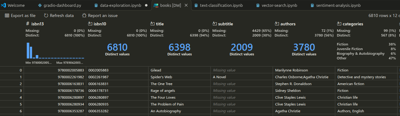
The first step you want to perform is to inspect your dataset. In the video, the instructor showed the capabilities that were present in PyCharm to natively inspect your dataset. It provided column headings with key statistics for each column and its data. Some of these metrics may include:

• Count of missing values
• Total Count
• Total Distinct values
• Top Values
• Frequency of values

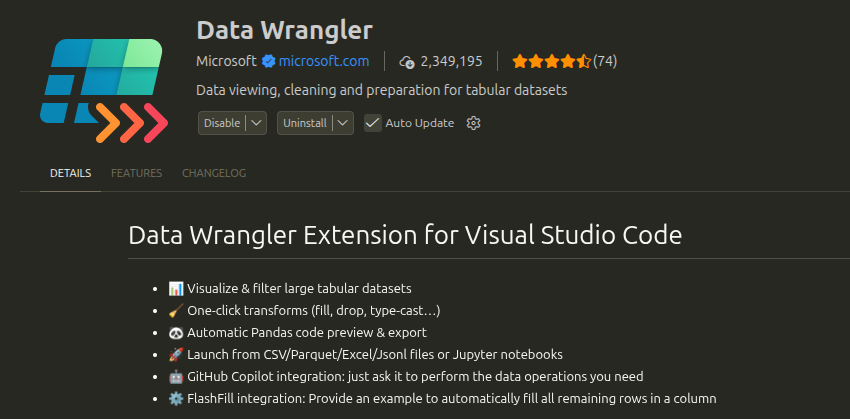
If you don't have PyCharm, don't worry because similar features exist in Visual Studio Code, and this is what I used to perform all of the operations for this tutorial. To get the same feature, Microsoft provides an extension to VS Code called Data Wrangler. This will provide mostly the same functionality with column heading metrics.

What are we looking for?

With all of the column header metrics available, what kind of features and metrics should we be looking for in this dataset?

• What useful data do we have?
• Patterns in missing values? Is there bias present?
• High levels of distinct values for categories and data that is meant to classify a subject.
• Values inconsistent with the rest of its cohort. Single word descriptions when all others are multiple lines for example.

Fixing Missing Values

As you are looking through your data you may notice that some columns have rows that are missing a value. While this might seem innocuous at first, you will want to understand if these missing values have any sort of pattern. A pattern of missing values could indicate some kind of bias in your dataset. Bias can introduce unwanted and inaccurate representations of your dataset that skew towards an unfair or even discriminatory outcome. So we want to make sure that we suss out any bias in our dataset.

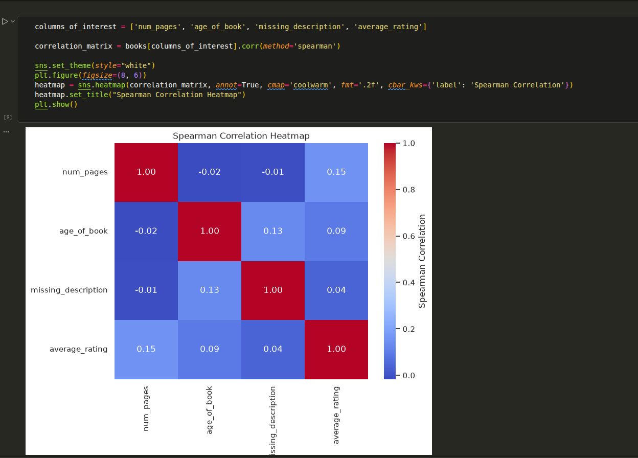
To find these in the dataset, the instructor of the video showed how to use seaborn and matplotlib to create a corelation heatmap. What this heatmap is able to show us is how relevant certain columns are to one another. As the corelation gets closer to 1 or -1, the corelation is strong and means there may be some bias with regards to the two related columns.

In this situation, there was no corelation, as the values were all closer to zero. So the missing values in the description fields do not have any pattern and don't indicate a bias.

Finding uninformative data values

Depending on how you are training your model, some data fields may require more informative data than others. When you have a specifically critical field that has some inconsistently small or uninformative values, like an incomplete book description (in this example), you will want to clean that up. But how can you find those data values easily enough and decide which are too small?

1. Build a dataframe that contains the count of rows based on their length (book description).
2. Inspect the dataframe to see the total distribution and get a sense of the upper value that will be the what is necessary to have a good description for our uses.
3. Filter based on some of the smaller distributions and inspect a sample of the descriptions. Read through a few to see if they have a good amount of data. Use your gut to understand what would be the best upper limit here.

While we can see here that there are some interesting features that we use to "scientifically" analyze the dataset, sometimes decisions have be made on a quality analysis also. A humans in the loop.

Additional Improvements

Once the data was cleaned up, there were a couple of small additions made to give the recommendation engine a little more to work with. The first was combining each book's title with its subtitle. A lot of books have a short, catchy title that doesn't tell you much on its own, and the subtitle is often where the real context lives. Joining the two into a single field gives us a fuller label for each book without having to juggle two separate columns.

The second was tagging each description with the book's ISBN. This might seem like an odd thing to do, but it pays off later on. When we start searching through the descriptions, every result that comes back will carry its ISBN along with it, so we can trace it straight back to the book it came from and filter on it efficiently. Neither of these changes is complicated, but they are a good example of how a little bit of thought during data preparation can save you a lot of work down the road.

Vector Search

With a clean dataset in hand, the next big step was building a vector database. This is the heart of the recommendation engine, because it lets us search the books by their meaning instead of matching on keywords. So if someone searches for "a story about forgiveness," they can get back books that deal with that theme even if the word "forgiveness" never shows up in the description.

So how does that work? A vector database stores an encoding of each piece of text, whether that's a whole document, a paragraph, or a single sentence. This encoding, called an embedding, is a vector representation of what the text means. The embeddings are created by an encoder model, and the video walked through RoBERTa as an example of this kind of model. Along with each embedding, the database stores an ID that points back to the original text. This is where tagging the descriptions with ISBNs during data preparation pays off, because every result we get back can be traced straight to the book it came from.

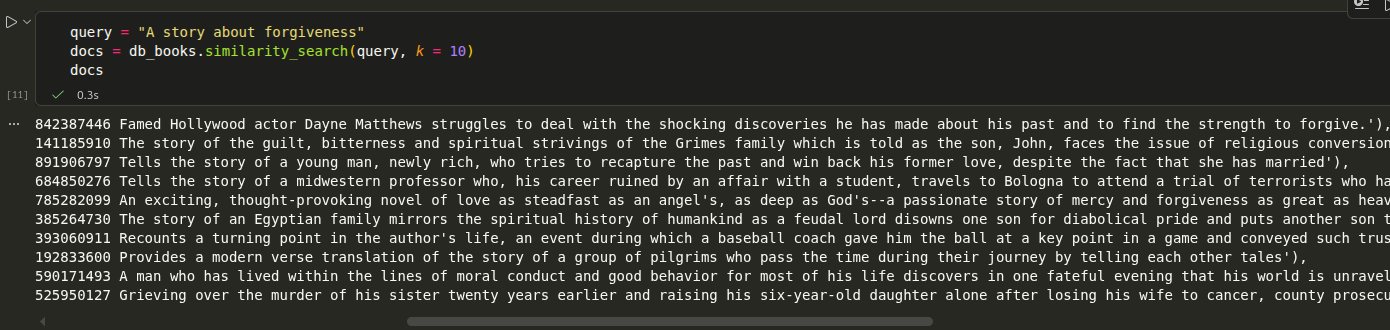
When you run a search, your query gets converted into an embedding using the same model. The database then compares that query vector against the vectors it has stored and retrieves the ones that are closest to it. Those results are ranked by how similar they are to your query, and that similarity is usually returned as a floating point score, where a higher number means a closer match. Texts with similar meanings end up close together in the vector space, which is why the search can pick up on themes and ideas rather than exact wording.

Comparing your query against every single vector in the database one by one, a linear search, gets expensive fast as the dataset grows. To get around this, vector databases build faster search techniques into their indexing system. These approaches trade a tiny bit of accuracy for a huge boost in speed by narrowing down where to look instead of checking everything. The nice part is that you don't have to build any of this yourself. It comes along for free when you use a vector database.

Classification

The next step in the tutorial was to classify each book into a broad category like Fiction or Non-fiction based on its description. This gives the recommendation engine another way to filter results, so if someone is looking for a novel they aren't handed a cookbook. The problem is that the dataset's existing categories were all over the place, and a good chunk of the books didn't have a useful category at all. So we needed a way to fill in those gaps.

To do this, the video used a zero-shot classification model. So how does that work? A zero-shot classifier doesn't need to be trained on your specific dataset. You hand it a piece of text (the book description in our case) along with a list of candidate labels, like "Fiction" and "Non-fiction", and it returns a score for how well each label fits. The label with the highest score wins. The model already has a general understanding of language baked in, so it can make a reasonable guess about which label fits a description it has never seen before.

Before running the classifier, though, there was some prep work to do. The books that already had a category were mapped into a smaller set of more general topics. For example, children's non-fiction just becomes non-fiction, and fantasy rolls up into fiction. These already-labeled books serve two purposes. First, they give us a set of known answers we can run the classifier against to see how accurate it really is before we trust it. Second, once we are happy with the accuracy, we can let the classifier loose on the rest of the corpus to fill in the books that were missing a category.

So what works well with this approach? Having a good-sized set of books that are already labeled with your categories, and that also have a decent description, makes a big difference. The more examples you have, the more confident you can be in the accuracy you are measuring. Rolling similar categories up into broader topics also helps, because the classifier has a much easier time picking between a handful of clearly different labels than a long list of overlapping ones.

What doesn't work so well are categories that are very niche and can't be folded into a larger category. The same goes for categories that just don't have enough labeled books with good descriptions behind them. If you only have a handful of examples, you have no real way of knowing whether the classifier is getting that category right. At the end of the day, the classifier is only as useful as the labeled data you have to check it against, which is another reason all that data cleaning up front was worth the effort.

Sentiment Analysis

The last piece of the tutorial added some emotional flavor to the recommendations. Using sentiment analysis, each book description was scored on the emotions it conveys, so a reader could ask for something suspenseful, joyful, or sad and get books that match the mood they are in. The video used a fine-tuned model to do this. So how does that work, and how is it different from an LLM or the zero-shot classifier we used in the last section?

The model measures seven emotions: anger, disgust, fear, joy, sadness, surprise, and neutral. It takes the text of the description as input, works out its semantic meaning, and outputs a probability for each of those seven labels. The higher the probability, the more strongly the description leans toward that emotion. What it doesn't do is predict the next token the way most LLMs do. It's built on an encoder-only transformer, so instead of generating text it reads the whole description at once and hands back a set of scores.

This is where it gets similar to the zero-shot classifier, and where the two part ways. Neither one needs to be trained on our book dataset. We just load the model and run our descriptions through it. The difference is in how each one knows its labels. The zero-shot classifier takes whatever labels you hand it at runtime, so you could swap "Fiction" and "Non-fiction" for any other set of categories. The emotion model was fine-tuned ahead of time on a dataset of text labeled with these specific seven emotions. Those labels are baked into the model, and you can't ask it about an emotion it wasn't fine-tuned on. The tradeoff is that it tends to do a better job at that one narrow task than a general-purpose model would.

Text classification vs Zero Shot Classification

This tutorial used both a zero-shot classifier and a fine-tuned text classifier, which made me want to dig into the differences between the two. Both take a piece of text and assign it a label, so at first glance they look like they do the same job. So why would you pick one over the other?

The biggest difference is where the labels come from. A fine-tuned text classifier is trained ahead of time on a dataset of text that has already been labeled. The labels it learns during that training are the only ones it knows, like the seven emotions in our sentiment model. A zero-shot classifier works the other way around. You give it the labels when you run it, and it uses its general understanding of language to decide which one fits best. If you want to change your categories tomorrow, a zero-shot classifier doesn't care. A fine-tuned classifier would need to be trained all over again.

That flexibility comes at a cost, though. Because a fine-tuned classifier has been trained specifically for its task, it will usually be more accurate at it than a zero-shot model that is making an educated guess. It also tends to be faster. Many zero-shot classifiers check each candidate label against the text one at a time, so the more labels you hand it, the longer it takes. A fine-tuned classifier scores all of its labels in a single pass. The catch is that fine-tuning requires a good amount of labeled data, and that labeled data is often the hardest part to come by.

So when should you use each one? A zero-shot classifier is a great fit when you don't have labeled data, when your categories are likely to change, or when you just want to try out an idea quickly before investing more time into it. That's exactly why it made sense for sorting our books into Fiction and Non-fiction. A fine-tuned text classifier is the better choice when your labels are stable and well defined, and when you either have plenty of labeled data or can find a model that someone else has already fine-tuned for your task. That's what happened with the emotion model. Someone had already done the hard work, so we got the benefits of a fine-tuned classifier without having to train anything ourselves.

These two don't have to be an either-or decision, either. A common approach is to start with a zero-shot classifier to get something working, use it to help build up a set of labeled data, and then fine-tune your own classifier once you have enough of it. You get up and running quickly and still end up with a more accurate model down the road.